compress model
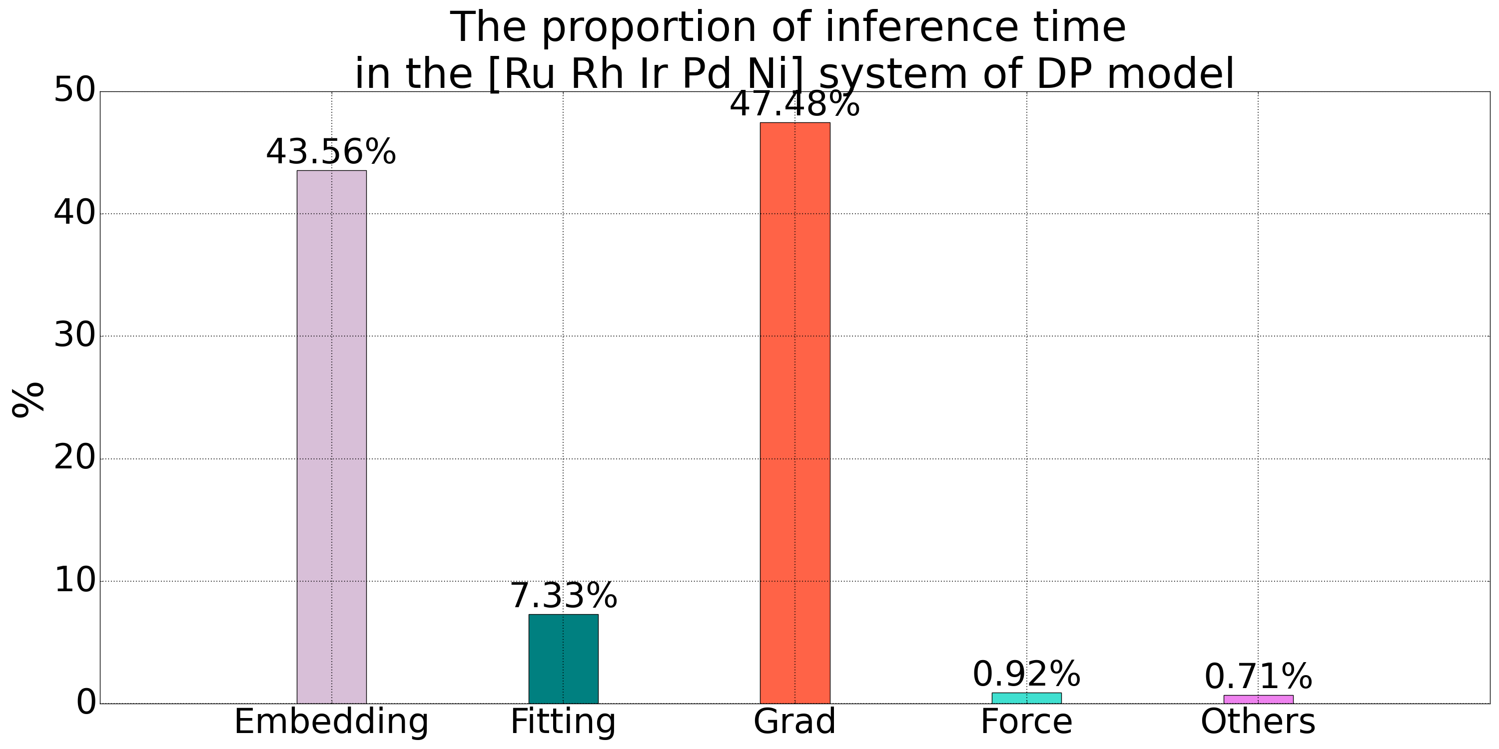
The number of Embedding net networks in the DP model is times the number of atom types . As the number of atom types increases, the number of Embedding net networks will rapidly increase, leading to a larger computational graph for backpropagation, which becomes one of the bottlenecks for inference in the DP model. The time statistics for the inference process of a quinary alloy system in the DP model show that the time spent on Embedding net computation and gradient calculation accounts for over 90% of the total time, indicating significant optimization potential.
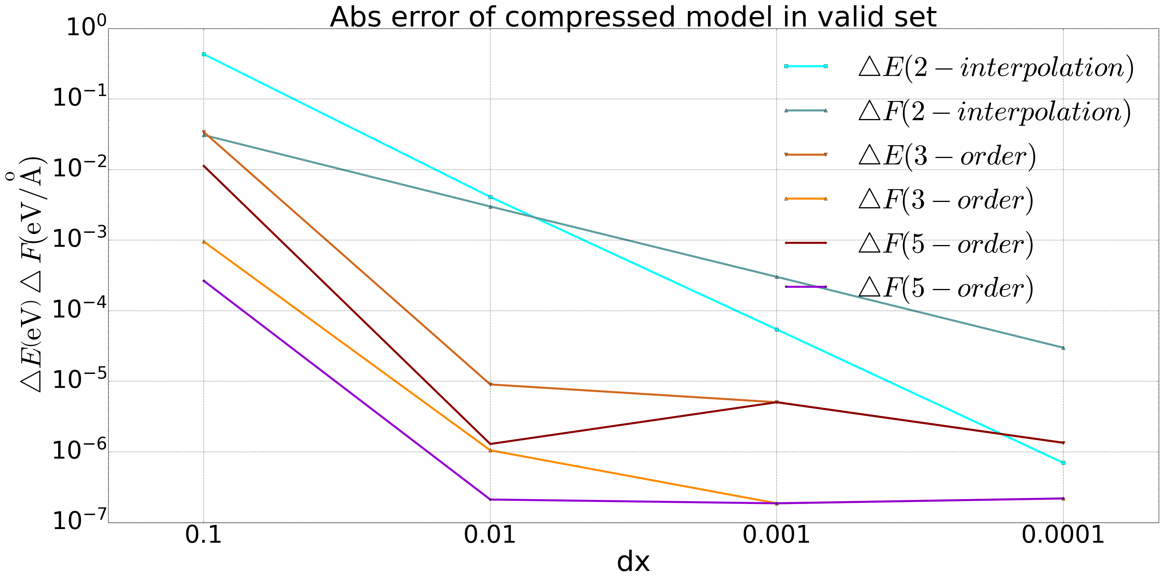
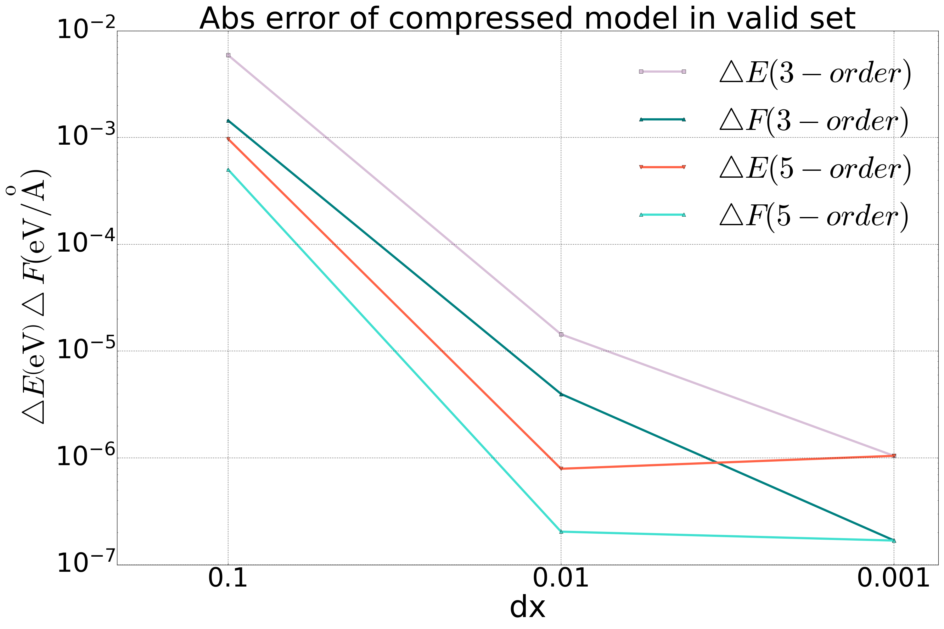
The input to the Embedding net is a single value of , and the output is a set of values (where is the number of neurons in the last layer of the Embedding net). Therefore, the Embedding net can be replaced by single-value functions. Here, we implement the fifth-order polynomial compression method described in the paper DP Compress, and we also provide the option of using the third-order polynomial compression method based on Hermite interpolation. In our tests, when the grid size , both the third-order and fifth-order polynomial compression methods achieve the same accuracy. Detailed test data can be found in the performance test.

Usage
To compress a trained DP model, the complete model compression command is as follows:
PWMLFF compress dp_model.ckpt -d 0.01 -o 3 -s cmp_dp_model
- "compress" is the command for compression.
- "dp_model.ckpt" is the name of the model file to be compressed and is a required parameter.
- -d specifies the grid partition size for . The default value is 0.01.
- -o determines the order of model compression. Use 3 for third-order model compression and 5 for fifth-order model compression. The default value is 3.
- -s sets the name of the compressed model. The default name is "cmp_dp_model".
After compressing the model, you can use it in molecular dynamics simulations in LAMMPS using the same approach as the standard DP model.
performance test
Model Compression Accuracy
We performed model compression on the DP model for both bulk copper and a quinary alloy system, and conducted tests on a valid set. The results are shown in the following figure. For the copper system, we included a comparison of accuracy using second-order interpolation, and it was found that the accuracy of the second-order method did not meet the required standards when compared to the third-order and fifth-order methods.
 Fig 1. Comparison of 2-order, 3-order, and 5-order polynomial compression in the DP model of Bulk copper system |  Fig 2. Comparison of 3-order and 5-order polynomial compression in the DP model of a five element alloy system |
speed
We conducted a statistical analysis of the inference time for the DP model with 3-order polynomial compression and the uncompressed model on the entire valid set of the quinary alloy system. After applying polynomial compression, there was a noticeable reduction in the time required for backpropagation (autograd). This is because the polynomial method significantly reduces the size of the computational graph for the Embedding net during automatic differentiation in PyTorch.
Fig 1. Comparison between with 3-order polynomial compression (dx=0.01) and uncompressed DP model for the quinary alloy system |
The compression process of 3-order polynomial
Grid partitioning of
We scan the entire training set to obtain the maximum value of . Since is a function of the 3-dimensional coordinate distance between atom and , we take the minimum value when . Based on the range of , we divide it into equal parts with a spacing of , resulting in a total of interpolation points denoted as . In practical usage, due to the incompleteness of the training set, there may be some values that exceed the range of the training set. In this case, we extend the grid beyond the aforementioned range and add values up to , with a grid size of .
3-order polynomial
For each interval , the Embedding net is replaced by the following third-order polynomial
Here, represents the number of neurons in the last layer of the Embedding net, which is the number of output values of the Embedding net. The . At each grid point, the following 2 conditions need to be satisfied. The polynomial values are consistent with the output values of the Embedding net.
The first derivative of the polynomial is consistent with the first derivative of the Embedding net with respect to .
The corresponding coefficients are determined as a result.
Where and .
5-order polynomial
We have also implemented the 5-order polynomial compression method described in DP Compress.
For the 5-order polynomial, the partitioning method for is the same as the 5-order method, and the following polynomial is used to replace the Embedding net
Here, represents the number of neurons in the last layer of the Embedding net, which is the number of output values of the Embedding net. The . At each grid point, the following 3 conditions need to be satisfied.
The value of the polynomial should be consistent with the output of the Embedding net.
The first derivative of the polynomial is consistent with the first derivative of the Embedding net with respect to .
The second derivative of the polynomial should match the second derivative of the Embedding net with respect to .
Consequently, we obtain 6 coefficient values, which are as follows.
Where and